Calculation of the flow rate of a rock-ramp pass

The calculation of the flow rate of a rock-ramp pass corresponds to the implementation of the algorithm and the equations present in Cassan et al. (2016)¹.

General calculation principle

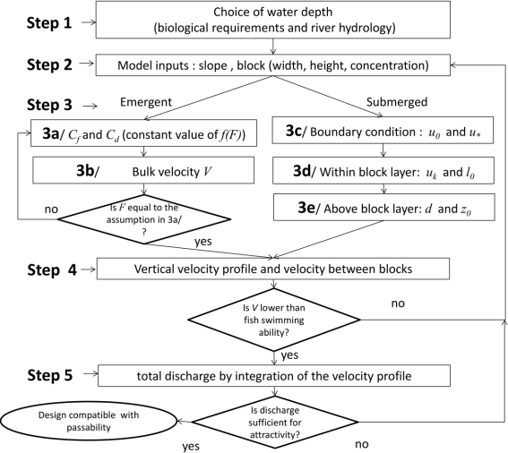
After Cassan et al., 2016¹

There are three possibilities:

• the submerged case when \(h \ge 1.1 \times k\)
• the emergent case when \(h \le k\)
• the quasi-emergent case when \(k < h < 1.1 \times k\)

In the quasi-emergent case, the calculation of the flow corresponds to a transition between emergent and submerged case formulas:

\[Q = a \times Q_{submerge} + (1 - a) \times Q_{emergent}\]

with \(a = \dfrac{h / k - 1}{1.1 - 1}\)

Submerged case

The calculation is done by integrating the velocity profile in and above the macro-roughnesses. The calculated velocities are the temporal and spatial averages per plane parallel to the bottom.

In macro-roughnesses, velocities are obtained by double averaging the Navier-Stokes equations in uniform regime with a mixing length model for turbulence.

Above the macro-roughnesses, the classical turbulent boundary layer analysis is maintained. The velocity profile is continuous at the top of the macro-roughnesses and is dependent on the boundary conditions set by the hydraulics:

• velocity at the bottom (without turbulence) in m/s:

\[u_0 = \sqrt{2 g S D (1 - \sigma C)/(C_d C)}\]

• total shear stress at the top of the roughnesses in m/s:

\[u_* = \sqrt{gS(h-k)}\]

The average bed velocity is given by integrating the flows between and above the blocks:

\[\bar{u} = \frac{Q_{inf} + Q_{sup}}{h}\]

with respectively \(Q_{inf}\) and \(Q_{sup}\) the unit flows for the part in the canopy and the part above the canopy.

Calculation of the unit flow rate Q_inf in the canopy

The flow in the canopy is obtained by integrating the velocity profile (Eq. 9, Cassan et al., 2016):

\[Q_{inf} = \int_{0}^1 u(\tilde{z}) d \tilde{z}\]

with

\[u(\tilde{z}) = u_0 \sqrt{\beta \left( \frac{h}{k} -1 \right) \frac{\sinh(\beta \tilde{z})}{\cosh(\beta)} + 1}\]

with

\[\beta = \sqrt{(k / \alpha_t)(C_d C k / D)/(1 - \sigma C)}\]

with

\[C_d = C_{x} f_{h_*}(h_*)\]

and \(\alpha_t\) obtained by solving the following equation:

\[\alpha_t u(1) - l_0 u_* = 0\]

with

\[l_0 = \min \left( s, 0.15 k \right)\]

with

\[s = D \left( \frac{1}{\sqrt{C}} - 1 \right)\]

Calculation of the unit flow Q_sup above the canopy

\[Q_{sup} = \int_k^h u(z) dz\]

with (Eq. 12, Cassan et al., 2016)

\[u(z) = \frac{u_*}{\kappa} \ln \left( \frac{z - d}{z_0} \right)\]

with (Eq. 14, Cassan et al., 2016)

\[z_0 = (k - d) \exp \left( {\frac{-\kappa u_k}{u_*}} \right)\]

and (Eq. 13, Cassan et al., 2016)

\[ d = k - \frac{\alpha_t u_k}{\kappa u_*}\]

which gives

\[Q_{sup} = \frac{u_*}{\kappa} \left( (h - d) \left( \ln \left( \frac{h-d}{z_0} \right) - 1\right) - \left( (k - d) \left( \ln \left( \frac{k-d}{z_0} \right) - 1 \right) \right) \right)\]

Emerging case

The calculation of the flow rate is done by successive iterations which consist in finding the flow rate value allowing to obtain the equality between the flow velocity \(V\) and the average velocity of the bed given by the equilibrium of the friction forces (bottom + drag) with gravity:

\[u_0 = \sqrt{\frac{2 g S D (1 - \sigma C)}{C_d f_F(F) C (1 + N)}}\]

with

\[N = \frac{\alpha C_f}{C_d f_F(F) C h_*}\]

with

\[\alpha = 1 - (a_y / a_x \times C)\]

Formulas used

Bulk velocity V

\[V = \frac{Q}{B \times h}\]

Average speed between blocks V_g

From Eq. 1 Cassan et al (2016)¹ and Eq. 1 Cassan et al (2014)²:

\[V_g = \frac{V}{1 - \sqrt{(a_x/a_y)C}}\]

Drag coefficient of a single block C_d0

\(C_{d0}\) is the drag coefficient of a block considering a single block infinitely high with \(F << 1\) (Cassan et al, 2014²).

It is 1 for a circular block and 2 for a flat-faced block.

The modifications made to \(f_{h_*}(h_*)\) in version 4.14.0 of Cassiopée lead to the use of a drag coefficient \(C_x\) calibrated on the results of the experiments for the calculation of \(C_d\):

\[ C_x = C_{d0}* 1.4917 -0.3914 \]

We have \(C_{x} = 1.1003\) for \(C_{d0}=1\) and \(C_{x} = 2.592\) for \(C_{d0}=2\).

Block shape coefficient σ

Cassan et al. (2014)², et Cassan et al. (2016)¹ define \(\sigma\) as the ratio between the block area in the \(x,y\) plane and \(D^2\). For the cylindrical form of the blocks, \(\sigma\) is equal to \(\pi / 4\) and for a square block, \(\sigma = 1\).

Ratio between the average speed downstream of a block and the maximum speed r

The value of this ratio is (\(r=1.1\)) for cylindrical blocks (Tran et al. 2016 [^3]), and (\(r=1.5\)) for flat-faced blocks (Cassan et al. (2014)², Table 2).

The formula used in Cassiopée allows to take into account shapes of intermediate blocks between circular and square shapes from the values of \(C_{d0} = 1.1\) for cylindrical blocks and \(C_{d0} = 2.6\) for blocks with flat faces:

\[ r = 0.4 C_{d0} + 0.7 \]

Froude F

\[F = \frac{V_g}{\sqrt{gh}}\]

Froude-related drag coefficient correction function f_F(F)

If \(F < 1.3\) (Eq. 5, Cassan et al., 2016)

\[f_F(F) = \mathrm{min} \left( \frac{\sigma}{1- (F^2 / 4)}, \frac{1}{F^{\frac{2}{3}}} \right)^2\]

else (The distinction is only numerical because \(1- (F^2 / 4)\) is not defined for \(F > 2\))

\[f_F(F) = F^{\frac{-4}{3}}\]

Maximum speed u_max

According to equation 19 of Cassan et al, 2014² :

\[ f_F(F) = \left( \dfrac{U_d}{V_g} \right)^2 \]

And equation 4:

\[ \frac{u_{max}}{V_g} = r \dfrac{u_d}{V_g} \]

It is deduced that :

\[ u_{max} = V_g r \sqrt{f_F(F)} \]

Drag coefficient correction function linked to relative depth f_h*(h_*)

The equation used in Cassiopeia differs slightly from Equation 20 of Cassan et al. 2014 ² and Equation 6 of Cassan et al. 2016 ¹. Indeed, recent experiments have shown a better correlation with the following formula :

\[ f_{h_*}(h_*) = \min \left((1 + 1 / h_*^2), 3 \right) \]

Coefficient of friction of the bed Cf

If \(k_s < 10^{-6} \mathrm{m}\) then we use Blasius' formula

\[C_f = 0.3164 / 4 * Re^{-0.25}\]

with

\[Re = u_0 \times h / \nu\]

Else (Eq. 3, Cassan et al., 2016 d'après Rice et al., 1998)

\[C_f = \frac{2}{(5.1 \mathrm{log} (h/k_s)+6)^2}\]

Notations

• \(\alpha\): ratio of the area affected by the bed friction to \(a_x \times a_y\)
• \(\alpha_t\): length scale of turbulence in the block layer (m)
• \(\beta\): ratio between drag stress and turbulence stress
• \(\kappa\): Von Karman constant = 0.41
• \(\sigma\): ratio between the block area in the plane X,y et \(D^2\)
• \(a_x\): cell width (perpendicular to the flow) (m)
• \(a_y\): length of a cell (parallel to the flow) (m)
• \(B\): pass width (m)
• \(C\): blocks concentration
• \(C_d\): drag coefficient of a block under current flow conditions
• \(C_{d0}\): drag coefficient of a block considering an infinitely high block with \(F \ll 1\)
• \(C_f)\): bed friction coefficient
• \(d\): displacement in the zero plane of the logarithmic profile (m)
• \(D\): width of the block facing the flow (m)
• \(F\): Froude number based on \(h\) and \(V_g\)
• \(g\): acceleration of gravity = 9.81 m.s^-2
• \(h\): average depth (m)
• \(h_*\): dimensionless depth (\(h / D\))
• \(k\): useful block height (m)
• \(k_s\): roughness height (m)
• \(l_0\): length scale of turbulence at the top of the blocks (m)
• \(N\): ratio between bed friction and drag force
• \(Q\): flow (m³/s)
• \(S\): pass slope (m/m)
• \(u_0\): average bed speed (m/s)
• \(u_*\): shear velocity (m/s)
• \(V\): flow velocity (m/s)
• \(V_g\): velocity between blocks (m/s)
• \(s\): minimum distance between blocks (m)
• \(z\): vertical position (m)
• \(z_0\): hydraulic roughness (m)
• \(\tilde{z}\): dimensionless stand \(\tilde{z} = z / k\)

---

1. Cassan L, Laurens P. 2016. Design of emergent and submerged rock-ramp fish passes. Knowl. Manag. Aquat. Ecosyst., 417, 45 ↩↩↩↩↩

2. Cassan, L., Tien, T.D., Courret, D., Laurens, P., Dartus, D., 2014. Hydraulic Resistance of Emergent Macroroughness at Large Froude Numbers: Design of Nature-Like Fishpasses. Journal of Hydraulic Engineering 140, 04014043. https://doi.org/10.1061/(ASCE)HY.1943-7900.0000910 ↩↩↩↩↩↩